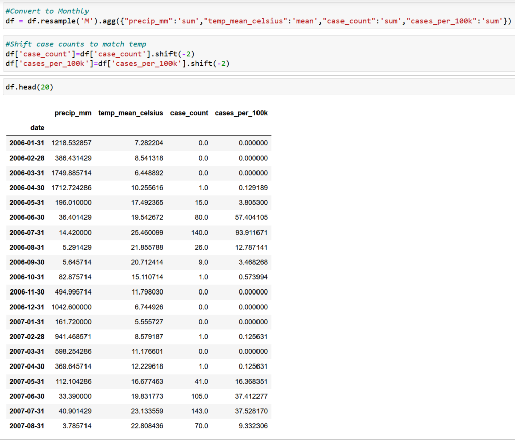
Based on our EDA in the previous post, we found that there is a two-month lag between temperature increase and the increase in our case_counts variable. To kick things off, we grouped the data by month and shifted the case_counts column up by two months so that the peak in temp_mean_celsius will match the peak in case_counts.
Now that are data is fully set up, we explored a number of models to find one that best fit our data. We have time series data that is inherently seasonal. We also ran an Augmented Dickey-Fuller Tests and found that our primary variables (temp_mean_celsius and case_count) are non-stationary, in that the statistical properties underlying the way in which the data changes over time are not constant.

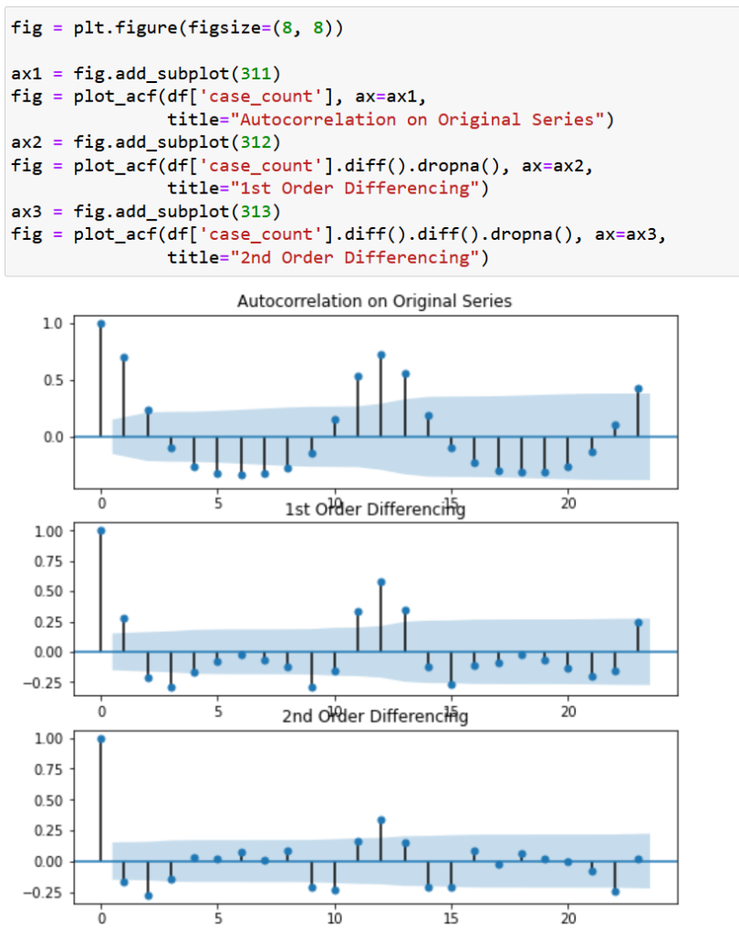
Furthermore, the two primary variables exhibited autocorrelation, in that observations were correlated with a previous observations. In other words, one observation in the time series is correlated with previous observations.
Given the complexity of the data, straightforward models such as linear regression would not be appropriate. We next examined an ARIMA model, which is designed for autocorrelated data, but we also needed to take seasonality into consideration. That brought us to the SARIMA, which is an ARIMA plus Seasonality. However, there was one last factor that we had to consider: exogeneous variables. In this case, using a SARIMA model would attempt to predict both case_counts and temp_mean_celsius based on past values. Instead, what we want is the model to take temperature as a input and predict case_count. Fortunately, the SARIMAX model (Seasonal ARIMA incl. eXogenous variables) was already a thing.
Without getting too much into the weeds, the ARIMA model (and its offshoots) seek to optimize three variables (p,d, and q) based on the data:
- p is the order (number of time lags) of the autoregressive model,
- d is the degree of differencing (the number of times the data have had past values subtracted), and
- q is the order of the moving-average model
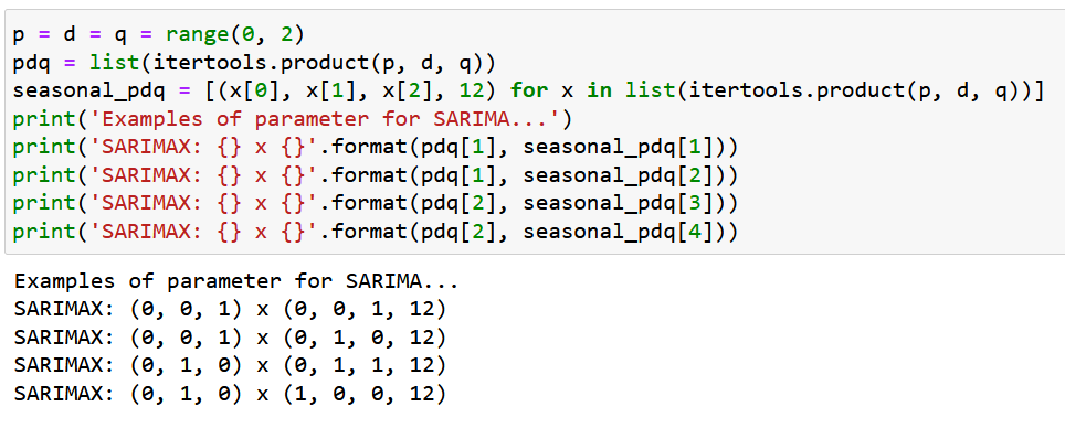
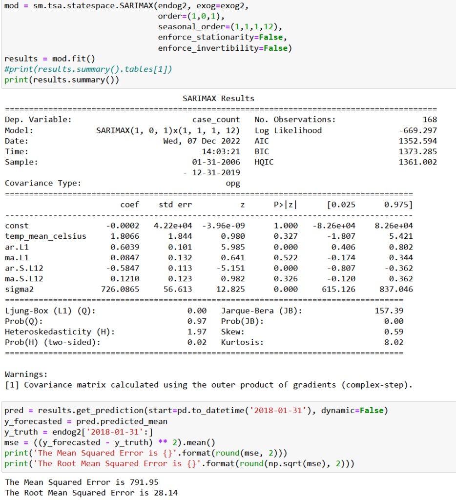
In addition to p, d, q, SARIMA(X) adds variables to account for seasonality. While there are ways to figure out the values of these variables yourself, it’s far easier to let python figure it out for you. The following blocks of code iterate through all of the possible combinations of p,d, q and seasonality and calculates the AIC ( a measure of statistical quality) for each combination.
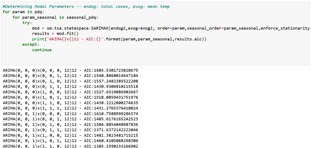
The above output is only a portion of the results. In general, the lower the AIC, the better, but the model error is also important. In Github, we built models based on the three combinations with the lowest AIC and calculated the Mean Squared Error (MSE) and Root Mean Squared Error (RMSE) for each model. In the case of MSE and RMSE, it’s also the lower the better. Below is the model with the lowest error values, which happened to be the third lowest AIC:
Based on data through 2017, we estimated the remaining two years so that we could compare the model’s predictions with actual data from 2018 onward. The blue line represents the actual case_counts numbers and the orange represents the model’s predictions:
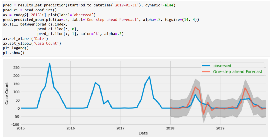
Based on the visuals, it turned out pretty well in that it matches the direction of the change, although it overestimates the magnitude at times. We did some additional numerical checks that are included on Github, and we felt that the model performed well enough to use it to predict the future.
Predicting the Future
One mistake often made in machine learning is attempting to predict for a period much longer than you have data for. Here we have about 5 years of data, so we sought to predict five years into the future. We also wanted to predict case_count based on a series of potential temperature scenarios: an increase of 0.5, 1, 1.5, 2 degrees celsius.
Recall that SARIMAX takes temperature as a given, so we also put together a table of temperature increases that we fed into the model.

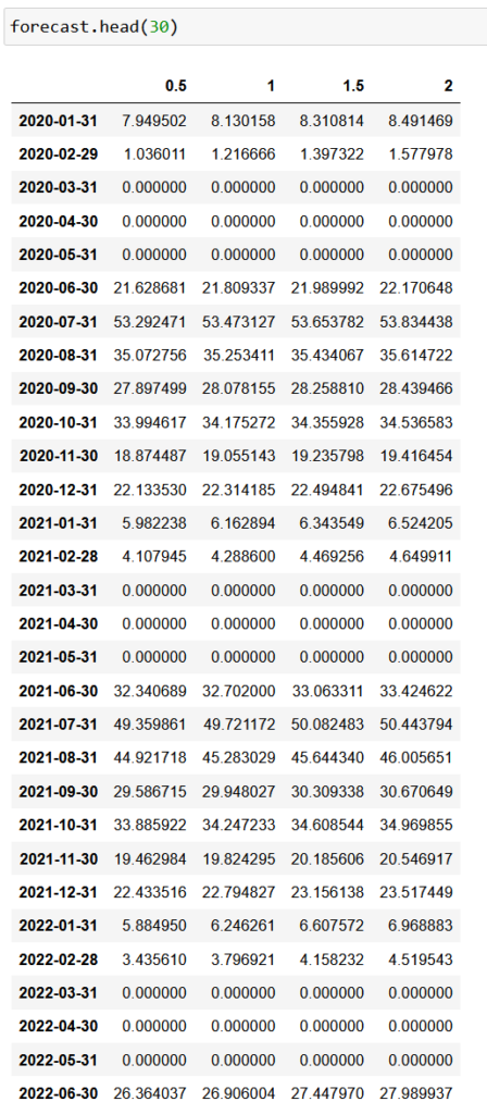
You’ll also notice in the above graph that in some instances, the model predicted negative case_counts, which doesn’t make any sense in the real world. This is a common concern with the SARIMAX model. Best practices in this case, is to set negative values to zero, which is what we did here. Below is the predicted case_counts for a one-half degree temperature increase:

Below are the results for the first 30 months of predictions under the 4 temperature scenarios:
Conclusion
That concludes this soup-to-nuts machine learning example. The purpose of this exercise to was demonstrate how complicated such an analysis can be and also that while it is a scientific process, there are many instances in which the data scientist must make a judgement call on which data to include, which model to use, and how to best structure the data. While that process is obviously not perfect, like everything else, one gets better at it with practice and experience.
As always, the entire code and data files are available on Github.
References
https://www.investopedia.com/terms/a/autocorrelation.asp
https://towardsdatascience.com/how-to-forecast-sales-with-python-using-sarima-model-ba600992fa7d
https://towardsdatascience.com/stationarity-in-time-series-analysis-90c94f27322