In this project, we will walk through the steps of building a predictive machine learning model. We will first begin with Data Cleaning, then move on to Exploratory Data Analysis (EDA), and in the third post, we will build, test, and fine tune our model.
In this ML example, we build a model to predict the prevalence of West Nile Virus in California over the next few years under a set of climate assumptions. The underlying hypothesis is that climate change will give rise to a higher incidence of West Nile Virus (WNV) in California, and we aim to predict the rate of infection under a series of scenarios ranging from mean temperature increase from 0.5 degrees Celsius to 2.0 degrees Celsius.
Data
This model will rely primarily on two publicly available datasets: WNV case counts by county and week provided by the California Health & Human Services Agency and daily climate data furnished by the PRISM Climate Group at Oregon State University. California is a big state with multiple climates, so we also incorporate geographic data to separate the state into regions.
The climate data consists of daily precipitation and temperature data, with a separate file for each county. The WNV data is a single file that tracks the number of cases by week for each county. The geographic data is simply the longitude and latitude for each county.
Climate Data
Importing the climate data posed two challenges. First, each of California’s 58 counties was housed in a separate csv file, which would need to be combined into a single dataframe. Secondly, the daily data will need to be converted to weekly data in order to match the WNV dataset.
Here, after setting a path where the files were located, we iterated through the folder to pull in the correct files, concatenate the data into one dataframe, simplify the column names, and pull in the name of each county from the file name.

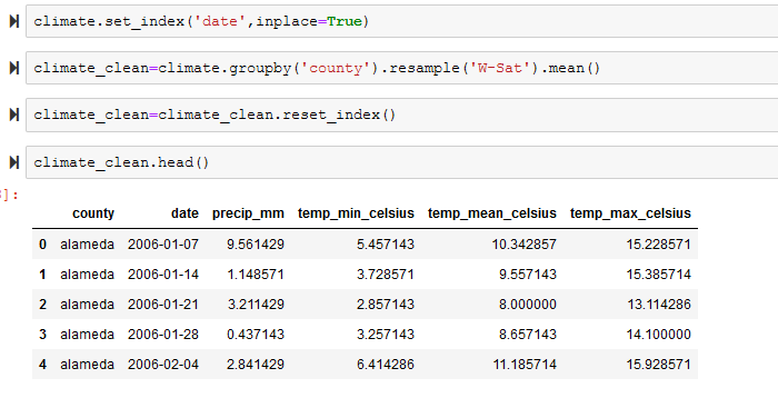
Next, we grouped the data by county and converted the daily data into weekly by taking the weekly mean for each feature based on the weekly structure in the WNV data.
WNV Case Count Data
The case count data is comprised of two datasets. The first is the counts per county per MMWR week, which is weekly numbering system devised by the CDC and used by several public health agencies. Generally, the first week of the year is MMWR Week 1, the second week is MMWR Week 2, and so on.

In order to match the WNV data with the climate dates, we also needed to pull in the dates that correspond to each MMWR week.

The MMWR week dates were listed horizontally, but we needed them vertically in order to merge them with the rest of the data. We used pandas melt function to transform the data from wide to long, turning the column headers into one column and matching up the MMWR week with the appropriate date for that year. And we also renamed the columns so that they would be easier to work with later.

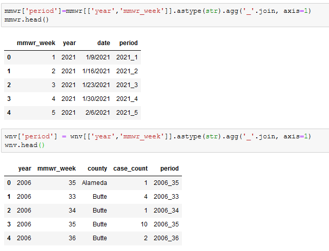
Once we had the MMWR weeks into a format that we wanted, we needed to merge the two dataframes to pull the MMWR dates into the WNV dataframe. In order to match the MMWR to the appropriate year, we needed unique identifier to merge on. We created a period column in both datasets, which is a concatenation of the year column and the mmwr_week columns.
We then merged the two datasets, adjusted the necessary data types and tidied things up a bit.

Combining Climate and WNV Data
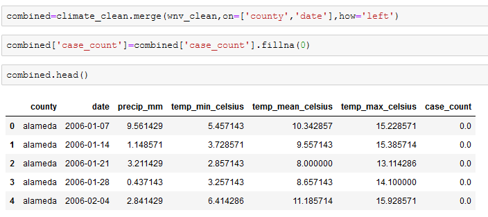
Our two primary datasets are now clean, formatted similarly, and are ready to be united. We created a new dataframe called combined, which merged the climate and WNV dataframes. Several counties had no WNV cases in certain weeks and this showed up as an NA in our wnv_clean dataframe. So after merging the two dataframes, we replaced the NAs with a 0 in the case_count column.
Geographic Coordinates
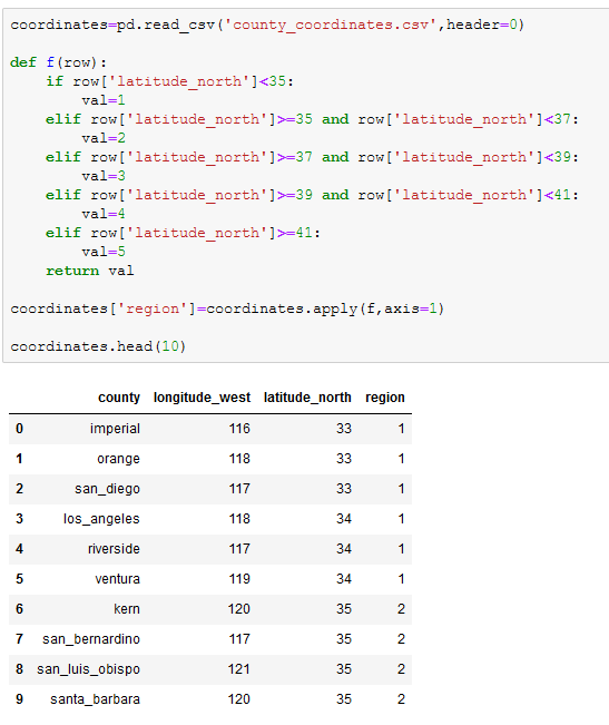
Thinking ahead to the analysis, we thought that examining the data by region could prove to be useful. We googled the longitude and latitude of each county and imported it as a new dataframe called coordinates. We then created a function to assign every two lines of latitude a regional number from 1 (north) to 5 (south).
As a final step, we merged the coordinates dataframe into the combined data frame that we created earlier.

This completes the data cleaning process. The complete python code can be found on GitHub. In our next post we’ll tackle Exploratory Data Analysis (EDA).